4.2 Data processing and analysis
To derive dependencies in complex critical infrastructure, in the case of use, i.e. subway infrastructure, the presented work uses sensitivity theory, which can be used to evaluate the strength of individual dependencies, i.e. their degree of vulnerability, which means the ability of dependencies to cause failure (KI, metro). The matrices are transformed into a graph for their subsequent analysis.
4.2.1 Theory of sensitivity
For reasons of better interpretation and work with information systems, vulnerability can also be defined as sensitivity using the theory of sensitivity [87,88], which can be queried by the following relationship [89]:

(22)
where Si is the absolute sensitivity of the output function y to the parameter of the input function xi. And according to source [90], in the sense of electronic systems, y = f(x1,..,,xi,…,xN) is a network (or system) function that depends on the circuit parameter xi. The change in the output function of the system is therefore dependent on its sensitivity and on the change in the input parameters xi, for practical reasons, the given relationship is written in matrix form, i.e. using the sensitivity matrix S [90]:

(23)
For electrical, electronic and programmable electronic systems (hereinafter referred to as E/E/PE), it is advantageous to calculate relative sensitivity and relative parameter change, as it enables the calculation of tolerances of the output quantity, the design of tolerances of input parameters, the optimization of the sensitivity of the electrical circuit, the search for the most sensitive elements, i.e. elements with the greatest influence on changes in the output quantity [90].
For working with assets, it is convenient to work with absolute sensitivity, because although the given scales for evaluating criticality are normalized, each function of the asset has a different physical basis.
4.2.2 Matrix notation and codification of names
It is common practice to list the relationships of individual elements in tables. In our case, it is sensitivity, i.e. the relationship between input variables (disasters, or assets) and output variables (system functions, or assets):
For better clarity, the matrix notation shown in Table 8 is used.
Table 8 Asset criticality table format for individual disasters.
| Disaster 1 | . … | Disaster n | |
| Asset 1 | S11 | . … | Sn1 |
| … | . | . … | . |
| Asset m | S1m | . … | Snm |
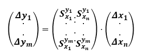
We convert Table 8 into matrix form, in which yi denotes assets and xi denotes calamities. Matrix notation makes it possible to perform appropriate operations and convert the matrix into a graph for scenario analysis.

(24)
The input parameters xi may actually also represent the output parameters of other assets (functions). In the event that we want to display the connections in more depth, by combining the input and output parameters on both sides of the equation, a concatenation can be created, i.e. for the purposes of the work, a “chained matrix of sensitivities”, which technically means the degree of vulnerability depending on the degree of connection of quantities or parameters [6 ,33].
In practice, the mentioned tables and matrices can take on large dimensions, and to ensure their readability, it is advisable to introduce an adequate codification of the names. The dissertation uses the numerical designation of disasters given in Appendix B. The used designation of asset groups is shown in Table 9.
Table 9 Asset group designations used.
| Group | Označení |
| Constructions | AK |
| Technik | AT |
| Staff | AP |
| Places | AM |
| Functions | AF |
| Connections and flows | AV |
| Organization and economics | AO |
The numerical designation of the subclasses of assets used below in the dissertation is given in Appendix C due to their large scale.
4.2.3 Transforming matrices into a graph
Using graph theory, described e.g. in [91], we can display vulnerabilities using a graded directed graph. To create a graph you need:
- use the sensitivities matrices, mentioned in the previous paragraphs 4.2.1 and 4.2.2,
- to transform sensitivity matrices into adjacency matrices, which express the degree of tightness of the connection of monitored quantities. The subject matrices are the basis for generating graphs that express the degree of connection of the relevant quantities.
The MS Excel tool is used to create adjacency matrices, the export of the matrix file is further imported into a tool designed for working with graphs – Gephi Data processing and analysis, tool: Gephi – The Open Graph See Platform version 9.0.2 [92].
The graph transformation process can be divided into the following steps:
- Compilation of adjacency matrices (a measure of connection tightness) from sensitivity matrices (a measure of vulnerability).
- Construction of an oriented graph – graphical interpretation.
- Evaluation of edges (vulnerability of a given link – connection) and nodes (vulnerability or criticality of monitored quantities, assets).
- Graph analysis and graphical interpretation of results.
4.2.3.1 Building adjacency matrices from sensitivity matrices
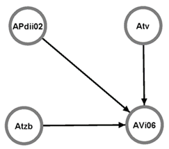
The adjacency matrix [91] expresses the relationship between two objects (in the given case, the input and output parameters of the function, or between nodes that represent assets or disasters). Their columns and rows represent the same set of objects in the same sequence. In order to be able to use sensitivity matrices, it is necessary to start with the input parameters of the function and then with the output parameters of the function as follows: APdii02; ATV; Atzb; AVi06 (notations used are explained in Appendix C).
According to matrix theory, we proceed by inserting a transposed sensibility matrix into the empty adjacency matrix and assuming that it is a basis for the construction of an oriented graph in which the relationships are one-way, we add zeros “0” to the other positions of the matrix. Table 10 represents the resulting adjacency matrix, the blue shaded table cells represent the transposed sensitivity matrix.
Table 10 Adjacency matrix for relation (44) (section 6.1.3).
| APdii02 | ATv | ATzb | AVi06 | |
| APdii02 | 0 | 0 | 0 | 1 |
| ATv | 0 | 0 | 0 | 1 |
| ATzb | 0 | 0 | 0 | 1 |
| AVi06 | 0 | 0 | 0 | 0 |
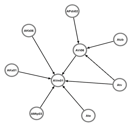
The subject algorithm can be applied to all previous simple relationships in which some input and output parameters are not common. For concatenated matrices, it is necessary to take into account common input and output parameters and create a sequence of nodes carefully. The concatenated matrix notation is shown in Table 11
Table 11 Adjacency matrix for concatenated matrices (relation (45) and 6.1.3).
| AKs01 | AKk06 | ATv | AVi06 | ATe | AMtp03 | APdii02 | ATzb | AVm01 | |
| AKs01 | 0 | 0 | 0 | 0 | 0 | 0 | 0 | 0 | 0,5 |
| AKk06 | 0 | 0 | 0 | 0 | 0 | 0 | 0 | 0 | 0,5 |
| ATv | 0 | 0 | 0 | 1 | 0 | 0 | 0 | 0 | 0,5 |
| AVi06 | 0 | 0 | 0 | 0 | 0 | 0 | 0 | 0 | 0,5 |
| ATe | 0 | 0 | 0 | 0 | 0 | 0 | 0 | 0 | 0,5 |
| AMtp03 | 0 | 0 | 0 | 0 | 0 | 0 | 0 | 0 | 0,5 |
| APdii02 | 0 | 0 | 0 | 1 | 0 | 0 | 0 | 0 | 0 |
| ATzb | 0 | 0 | 0 | 1 | 0 | 0 | 0 | 0 | 0 |
| AVm01 | 0 | 0 | 0 | 0 | 0 | 0 | 0 | 0 | 0 |
4.2.3.2 Construction of an oriented graph – graphical interpretation
According to the definition [91], a directed graph is expressed by an ordered triple:

(25)
where H is the set of edges, U is the set of nodes and σ is the incidence relation expressed by:

(26)
where u is the start vertex and v is the end vertex. The graph G can be fully derived from adjacency matrices [91]. The graph for Table 10 is in Figure 13 and for Table 11 is in Figure 14.

Figure 13. Graph for Table 3 (AVi06), [3].

Figure 14. Graph for Table 4 (Avi06-m01), [3].
4.2.3.3 Evaluation of edges (vulnerability of a given link) and nodes (vulnerability or criticality)
Figures 13 and 14 show graphs according to the mentioned adjacency matrices, but do not represent the assessment of edges and node parameters. For each edge and node, the required information can be attached to the text (evaluation using the weight of the edge, or the vulnerability or criticality of the node). With the use of the SW tool [92], the mentioned parameters can be interpreted graphically in different ways, i.e. changing the size or color of edges and nodes according to their properties.
For the purposes of the presented thesis, the weight of the edge is the degree of connection, or the degree of sensitivity (or vulnerability) of the target asset to the input parameter (function of the asset or disaster).
The textual evaluation of nodes in the dissertation shows the criticality if needed for the given analysis (e.g. Figure 21 in paragraph 6.2.3).
The dimensions and colors of the nodes and edges used in the thesis are described in the following paragraph.
4.2.3.4 Graph analysis and graphical interpretation of results
The Gephi 0.9.2 tool [92] was used to display the graph. The default display (layout) of nodes on the desktop in the tool is not ideal, so the layout must be adjusted accordingly. You can use the manual deployment of nodes according to the need and type of node or it is also possible to use known algorithms. At the same time, the color resolution of nodes and edges and their size should be adjusted according to their degree, weights and other parameters.
For graph analysis, the following settings of optional parameters, which the tool allows, were chosen [92]:
- Layout: force-oriented Fruchterman-Reingold [93], area: 10000; gravity: 10; speed 1, which will affect the resulting distribution of nodes and edges on the work surface (or on the canvas) in the SW tool.
- Nodes: size according to “Steps in”; min: 10; max: 50; exponentially, the specified setting on the desktop will exponentially grow nodes that have more incoming edges,
- color according to “Steps in”; min: black; max: red; linearly, the specified setting on the desktop will color red the nodes that have more incoming edges,
- “degree in” expresses the number of edges entering a given node, regardless of their weight,
- “degree out” expresses the number of outgoing edges from a given node, regardless of their weight.
- Edges: by default thickness by weight, color according to “Libra”; min: black; max: red; linearly distributed in the interval between minimum and maximum.
